卷積、相關（matlab）

本次博客主要是**圖示化卷積**過程，可以進一步加深學者在學習過程當中對數學卷積的理解。首先，再次回顧

一下利用MATLAB產生指數序列 x[k]=Kαku[k]，

a=input('a=');
K=input('K=');
N=input('N=');
k=0:N-1;
x=K*a.^k;
stem(k,x);
xlabel('Time');ylabel('Amplitude');
title(['\alpha=',num2str(a)]);

本博客中令a,K,N分別爲0.8，2，31；實驗產生的圖形爲

離散序列的卷積和相關是數字信號處理中的基本運算，MATLAB提供了計算卷積和相關的函數conv和xcorr，調用方式是：

y = conv (x, h)

y = xcorr (x, h)

x, h：分別爲參與卷積和相關運算的兩個序列；

y：返回值是卷積或相關的結果；

下面利用MATLAB函數 conv 計算x = [−0.5, 0, 0.5, 1]，h = [1, 1, 1]這兩個序列的卷積

x = [-0.5, 0, 0.5, 1]; kx = -1:2;
subplot(311),stem(kx,x);
h = [1, 1, 1]; kh = -2:0;
subplot(312),stem(kh,h);
y = conv (x, h);
k = kx(1)+kh(1) : kx(end)+kh(end);
subplot(313),stem (k, y);
xlabel ('k'); ylabel ('y');

在此處要注意一下k的取值範圍：

k =

-3    -2    -1     0     1     2

接下來再利用MATLAB函數 xcorr 計算x = [−0.5, 0, 0.5, 1]，h = [1, 1, 1]這兩個序列的相關。

x = [-0.5, 0, 0.5, 1]; kx = 0:3;
subplot(311),stem(kx,x);
h = [1, 1, 1, 1]; kh = 0:3;
subplot(312),stem(kh,h);
y = xcorr (x, h);
k = kx(1)-kh(end) : kx(end)-kh(1);
subplot(313),stem (k, y);
xlabel ('k'); ylabel ('y');

            ![](https://img2018.cnblogs.com/blog/1546658/202002/1546658-20200222001256455-1008028989.jpg)

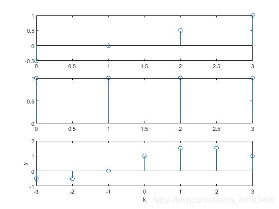
在此處要注意一下k的取值範圍：

k =

-3    -2    -1     0     1     2     3


再利用MATLAB函數 xcorr 計算x =[1, 1, 1]，h =  [−0.5, 0, 0.5, 1]這兩個序列的相關（即交換上面

那個例子倆序列的順序）

自相關

利用MATLAB函數 xcorr 計算x = [−0.5, 0, 0.5, 1]的自相關

x = [-0.5, 0, 0.5, 1]; kx = 0:3;
subplot(311),stem(kx,x);
h= [-0.5, 0, 0.5, 1]; kh = 0:3;
subplot(312),stem(kh,h);
y = xcorr (x, h);
k = kx(1)-kh(end) : kx(end)-kh(1);
subplot(313),stem (k, y);

同理可得x = [1，1，1， 1]的自相關

結果分析部分

從數字信號處理的角度方面來看，自相關運算能夠用卷積運算來代替；在此我就不擺複雜公式了，簡單的列舉

幾個結論；

自相關函數：r[-n]=r[n] 偶對稱序列，關於x=0對稱；能夠用xcorr[-n]=xcorr[n]表示；

r[n]在n=0處的數值最大；

互相關函數xcorr[X,Y]=-xcorr[Y,X]，可見xcorr[X,Y]與xcorr[Y,X]互爲其翻轉序列。